Reports, logs & plots

Once a calculation has converged, three complementary outputs help you inspect and archive it: a final text report, a per-iteration log, and publication-style plots.

Setup

This continues the running example (each manual page is self-contained, so we solve it again here):

using AtomicKohnSham
using Libxc

model = KSEModel(Z = 11, N = 11, ex = Functional(:lda_x; n_spin = 1), ec = NoFunctional(1))
mesh = expmesh(0, 500, 60; s = 1.2)
basis = P1IntLegendreBasis(mesh; ordermax = 10)
discretization = KSEDiscretization(basis, model; lh = 2, nh = 10,
    fem_integration_method = GaussLegendre(basis, 2000))
alg = ODA(tinit = 0.6, aufbau = OptimizedAufbau(max_degen = 2, tol = 1e-1), scftol = 1e-9)

sol = groundstate(model, discretization, alg; maxiter = 100)

`results.txt`: a final report

AtomicKohnSham.write_report — Function

write_report(sol::KSESolution, path::AbstractString)

Write a self-contained text report of a converged (or stopped) Kohn–Sham computation to path.

The report describes:

the run's identity and outcome (name, success flag, number of iterations, final stopping criterion),
every parameter used to define the computation (model, discretization, algorithm), read from sol.context,
the final energy decomposition,
the occupied orbitals with their energies and occupation numbers.

Arguments

sol::KSESolution: Solution returned by groundstate.
path::AbstractString: Destination file path (typically "results.txt").

source

write_report(sol, "results.txt")
print(read("results.txt", String))

Name    = Sodium
Success = SUCCESS
niter   = 20
Final stopping criterion = 5.569658855746759e-10
Data type = Float64

PARAMETERS
----------
  Model
    Z (nuclear charge)     = 11
    N (electrons)          = 11
    Hartree coefficient    = 1
    Exchange functional    = Slater exchange
    Correlation functional = None
    Spin channels          = 1

  Discretization
    Angular momentum cutoff (lh) = 2
    Orbitals per channel (nh)    = 10
    Basis                        = P1IntLegendreGenerator (ordermax = 10)
    Number of basis functions    = 589
    Mesh                         = Exponential Mesh (s = 1.2,)
    Rmax                         = 500.0
    Number of mesh points        = 60
    Integration method           = GaussLegendre (npoints = 2000)

  Algorithm = ODA
    scftol     = 1.0e-9
    tinit      = 0.6
    frozen_t   = false
    maxiter_ls = 100
    abstol_ls  = 2.220446049250313e-12
    reltol_ls  = 2.220446049250313e-12
    Aufbau = OptimizedAufbau
      max_degen               = 2
      tol                     = 0.1
      handle_degen_spin_1iter = true

ENERGIES
--------
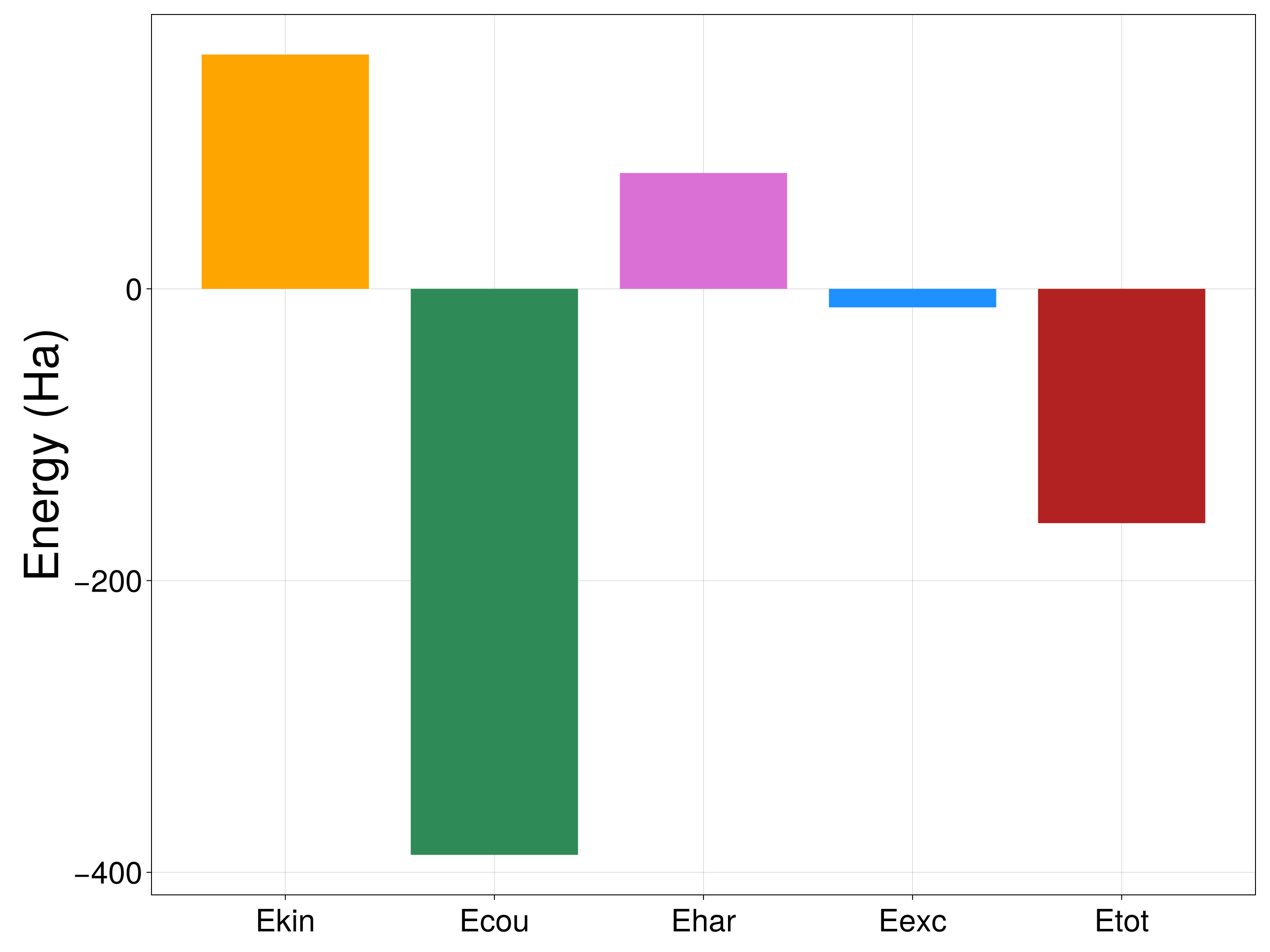
  Ekin (kinetic)              = 160.62822758864036
  Ecou (nuclear attraction)   = -388.0065460113607
  Ehar (Hartree)              = 79.43155311453171
  Eexc (exchange-correlation) = -12.681462279485856
  Etot (total)                = -160.6282275876745

OCCUPIED ORBITALS
-----------------
Occupation number =
            1s : ε = -3.764758179762527e+01        n = 2.0
            2s : ε = -2.007737456192821e+00        n = 2.0
            2p : ε = -1.006028994917961e+00        n = 6.0
            3s : ε = -7.701608708314467e-02        n = 0.999999999991612
            3p : ε = -1.111637722765135e-02        n = 8.387956995647983e-12

`log.txt`: per-iteration diagnostics

Rather than a verbosity flag on the solver, per-iteration diagnostics are written through the same CallbackSet mechanism used for any other callback — so log.txt keeps being updated even if the SCF loop is later interrupted or throws:

AtomicKohnSham.CallbackSet — Type

CallbackSet

Composite callback container.

Groups multiple callbacks into a single object. At each SCF iteration, all registered callbacks are executed sequentially.

source

AtomicKohnSham.LogFileCallback — Type

LogFileCallback(io::IO)

Callback that appends one line per SCF iteration to io, meant to be combined into a CallbackSet and passed to groundstate/KSESolver via the callback keyword. This replaces ad-hoc redirect_stdout logging: io is owned and closed by the caller, and logging keeps working even if the SCF loop throws.

Example

open("log.txt", "w") do io
    write_log_header(io, model, alg, dis)
    sol = groundstate(model, dis, alg; maxiter = 100,
                       callback = CallbackSet((LogFileCallback(io),)))
end

source

AtomicKohnSham.write_log_header — Function

write_log_header(io::IO, model::KSEModel, alg::SCFAlgorithm, discretization::KSEDiscretization)

Write the parameter block (identical to the one in write_report) at the top of a log.txt file, before the per-iteration lines appended by LogFileCallback.

source

open("log.txt", "w") do io
    write_log_header(io, model, alg, discretization)
    groundstate(model, discretization, alg; maxiter = 100,
        callback = CallbackSet((LogFileCallback(io),)))
end

lines = split(read("log.txt", String), "\n")
println(join(lines[1:12], "\n"))     # header
println("[...]")
println(join(lines[end-4:end-1], "\n"))  # final iterations

PARAMETERS
----------
  Model
    Z (nuclear charge)     = 11
    N (electrons)          = 11
    Hartree coefficient    = 1
    Exchange functional    = Slater exchange
    Correlation functional = None
    Spin channels          = 1

  Discretization
    Angular momentum cutoff (lh) = 2
[...]
iter = 16   stop = 6.123195518566815e-8   Etot = -160.6282275876745   Ekin = 160.62822766652363   Ecou = -388.0065461412495   Ehar = 79.43155317337806   Eexc = -12.681462286326735   t = 0.3819660112501051
iter = 17   stop = 1.278862503971953e-8   Etot = -160.62822758767453   Ekin = 160.6282276046341   Ecou = -388.00654603805646   Ehar = 79.43155312662408   Eexc = -12.68146228087626   t = 0.3819660112501051
iter = 18   stop = 2.6598166420803435e-9   Etot = -160.62822758767456   Ekin = 160.62822759149756   Ecou = -388.00654601613144   Ehar = 79.43155311668835   Eexc = -12.681462279729033   t = 0.3819660112501051
iter = 19   stop = 5.569658855746759e-10   Etot = -160.6282275876745   Ekin = 160.62822758864036   Ecou = -388.0065460113607   Ehar = 79.43155311453171   Eexc = -12.681462279485856   t = 0.3819660112501051

Plots

Plotting is a package extension: the plotting functions become available as soon as CairoMakie is loaded alongside AtomicKohnSham, with no extra setup:

using AtomicKohnSham, CairoMakie

AtomicKohnSham.plot_density — Function

plot_density(sol::KSESolution, X)
plot_density(sols::AbstractVector{<:KSESolution}, X)

Plot the radial electron density (log scale) on the radial points X, for one solution or several overlaid. Requires using CairoMakie.

source

AtomicKohnSham.plot_orbitals — Function

plot_orbitals(sol::KSESolution, X; l = nothing)

Plot the occupied Kohn–Sham orbitals, each shifted to its orbital energy and overlaid on the effective potential of its angular momentum channel (see eval_effective_potential). Restrict to a single channel with l. Requires using CairoMakie.

source

AtomicKohnSham.plot_potentials — Function

plot_potentials(sol::KSESolution, X; l = 0, σ = 1)

Plot the nuclear, Hartree, exchange–correlation, and centrifugal contributions to the effective potential of channel l, together with their sum. Requires using CairoMakie.

source

AtomicKohnSham.plot_convergence — Function

plot_convergence(sol::KSESolution)

Plot the SCF stopping criterion and the total-energy convergence (|Etot_i - Etot_final|) against iteration, both on a log scale. Requires using CairoMakie.

source

AtomicKohnSham.plot_energy_breakdown — Function

plot_energy_breakdown(sol::KSESolution)

Bar chart of the energy decomposition (Ekin, Ecou, Ehar, Eexc, Etot). Requires using CairoMakie.

source

Density

X = AtomicKohnSham.exprange(1e-3, 300, 2000; s = 1.5)
save("density.png", plot_density(sol, X))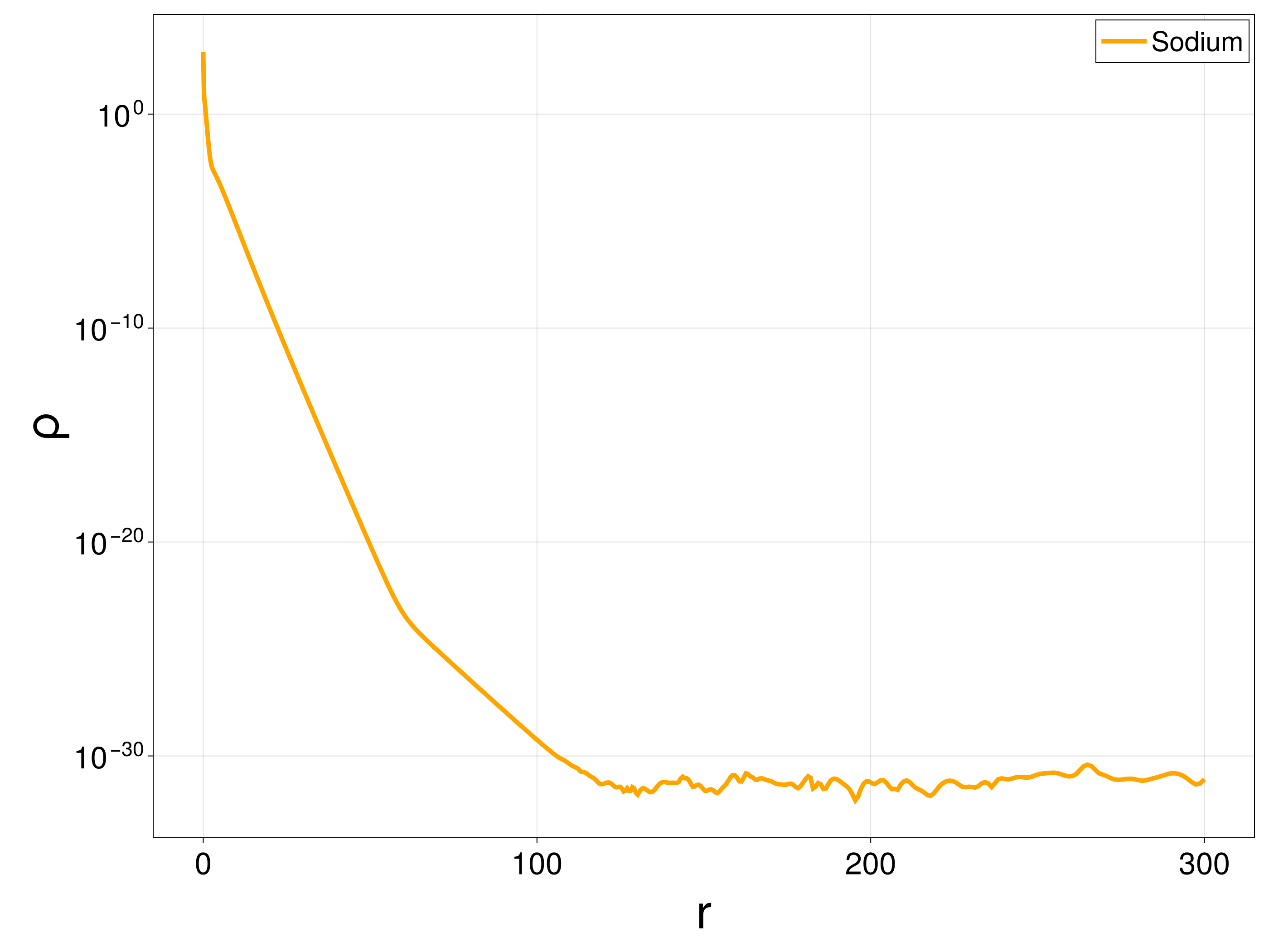

density

Orbitals

Each occupied orbital is drawn at its own energy, overlaid on the effective potential of its angular momentum channel (one panel per l):

save("orbitals.png", plot_orbitals(sol, X))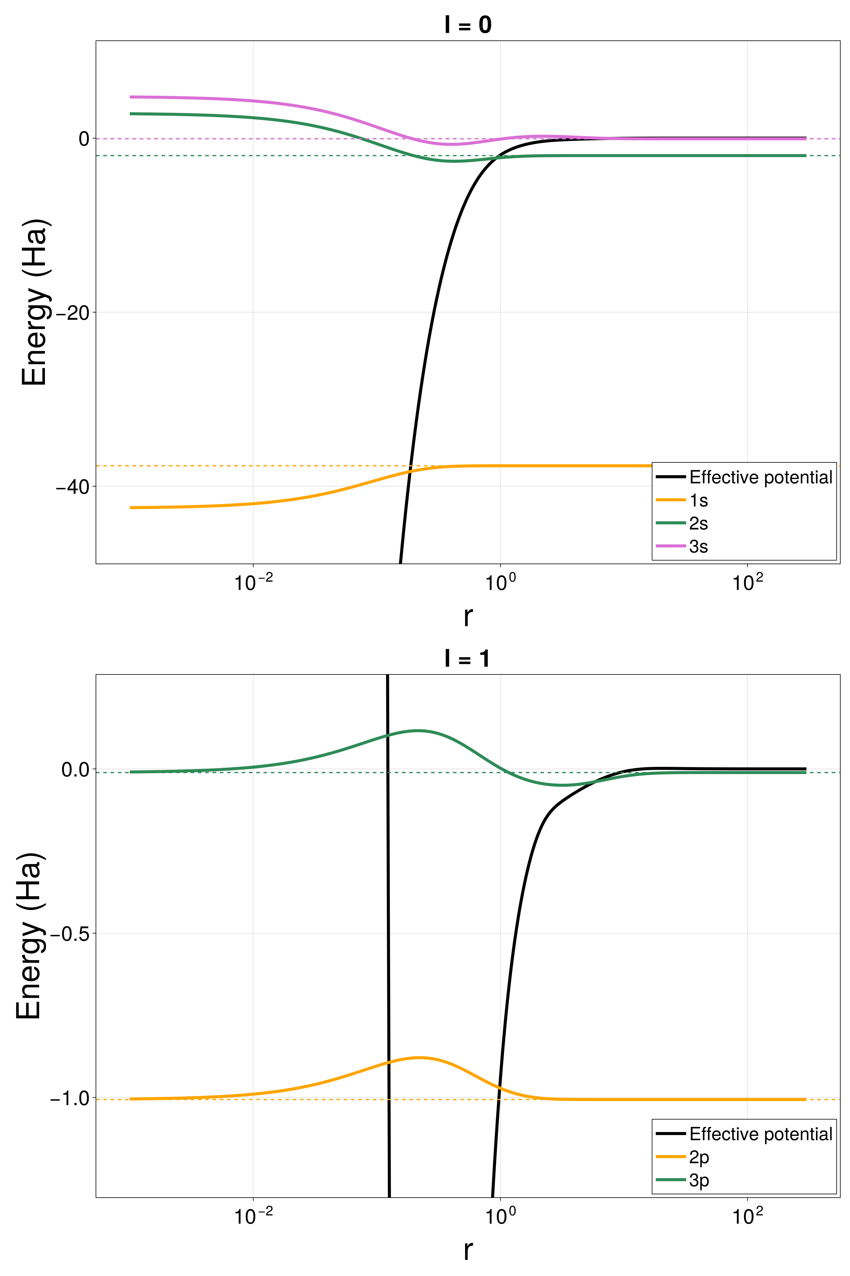

orbitals

Potentials

save("potentials.png", plot_potentials(sol, X; l = 0))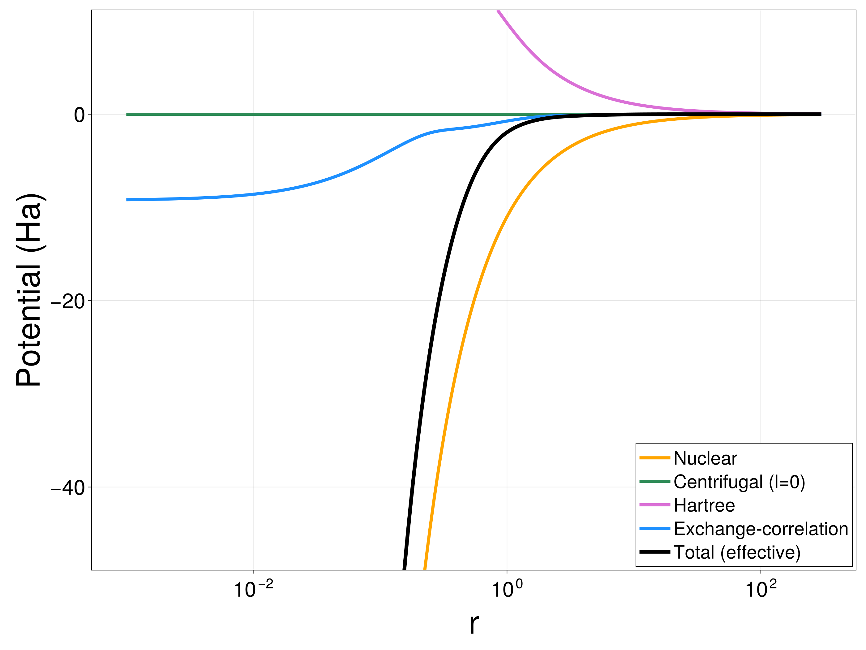

potentials

Convergence and energy breakdown

save("convergence.png", plot_convergence(sol))
save("energy_breakdown.png", plot_energy_breakdown(sol))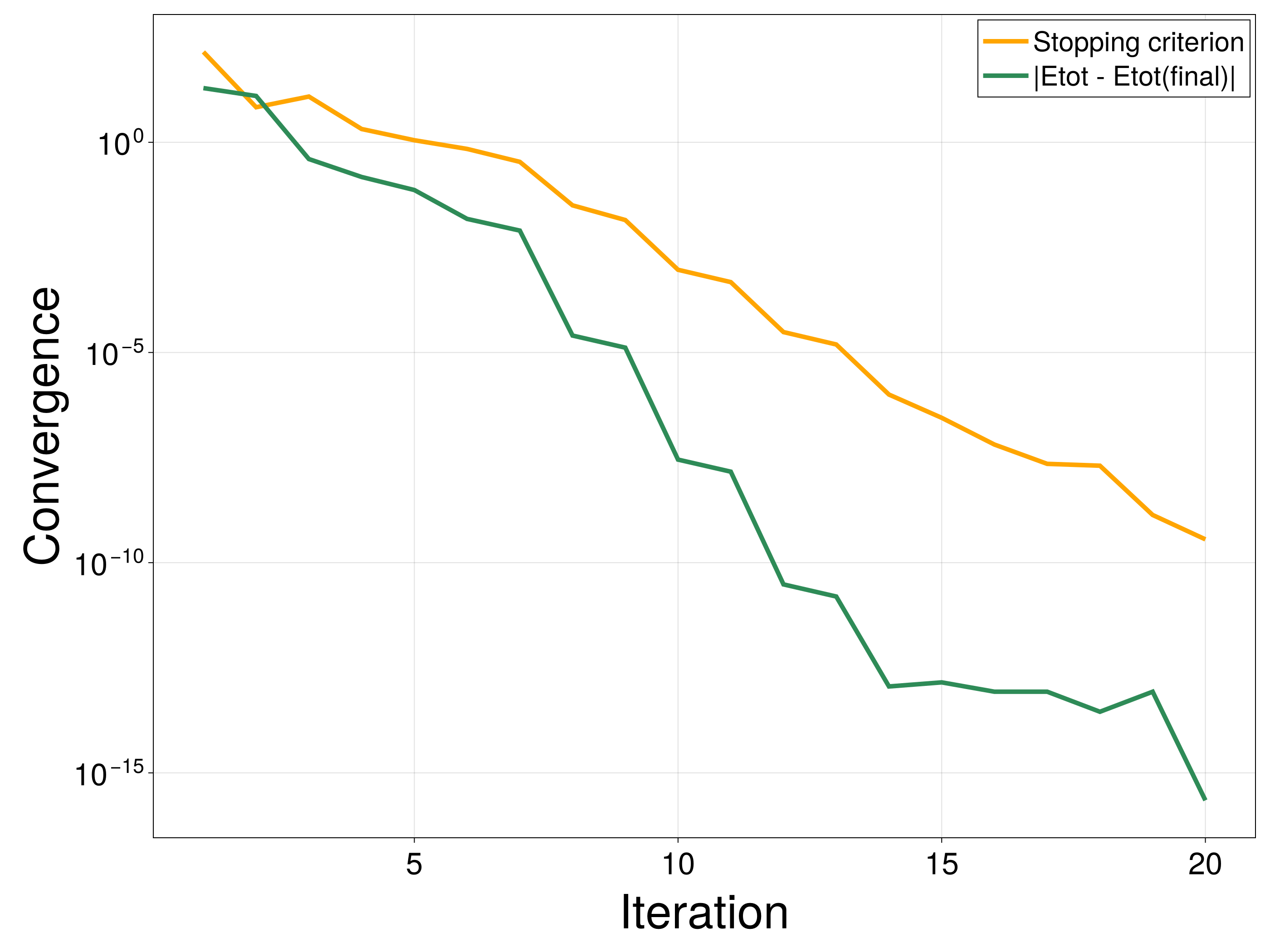

convergence energy breakdown

See the API Reference for the complete function index.